

Sudipta Deb
Founder of Technical Potpourri, Co-Founder of Shrey Tech, Enterprise Cloud Architect
A probability distribution specifies the likelihood of all possible outcomes of a random variable. The distribution may be classified as either continuous or discrete based on the values assumed by a random variable. Various forms of probability distributions exist. In this post, I will examine Normal, Binomial, Poisson and Bernoulli distribution and demonstrate how to utilize Python to plot it.
Regardless of your domain, Statistics and Probability will be there. Economics, finance, trading, social sciences, natural sciences, and data science are essential. A substantial portion of data science involves comprehending the behaviors and characteristics of variables, which necessitates knowledge of their corresponding distributions. The probability distribution is a method to depict the potential values a variable may assume along with their corresponding probabilities.
In this blog post, I will show you how to use the Python programming language to plot these 4 distributions.
The form you have selected does not exist.
Let's Understand Probability Distribution
A probability distribution is a function in probability theory and statistics that quantifies the likelihood of various outcomes in an experiment. It delineates occurrences based on their probability relative to all potential outcomes.
Let's say, the probability distribution of a fair coin toss. Heads takes a value of X = 0.5 and tails gets X = 0.5 too.
Understand Density Function
Another important thing to understand is the density function. The density functions are mathematical functions that describe the probability distribution of a random variable X. We have two density functions - Probability Mass Function (PMF) and Probability Density Function (PDF).
Probability Mass Function (PMF)
Describes the probability distribution of a discrete random variable.
- The number of heads in 3 coin flips (can be 0, 1, 2, or 3).
- The number of cars passing a point on a road in an hour.
Probability Density Function (PDF)
Describes the probability distribution of a continuous random variable.
- The temperature of city.
- A person's weight.
- The time it takes to fix a bug.
Let's Start With Normal Distribution
The Normal Distribution is a probability distribution that is symmetric around its mean value. It is a continuous distribution with two parameters: mean (μ) and standard deviation (σ). The bell-shaped curve of the Normal Distribution shows that most of the data falls near the mean, while the tail shows that there is still a chance for data to fall from the mean.
I have written a dedicated blog post covering Normal Distribution. So instead of duplicating the content, I am linking the blog post where you can get all the details you need about Normal Distribution.
Blog Post - Normal Distribution Using Python and SciPy
GitHub Code - NormalDistribution.ipynb
Now It's Time For Binomial Distribution
The binomial distribution is a discrete probability distribution that describes the probability of obtaining a certain number of successes
The binomial distribution is based on a series of independent trials called Bernoulli trials. Each Bernoulli trial has only two possible outcomes, conventionally labeled "success" and "failure." The probability of success is denoted by p, and the probability of failure is denoted by q = 1 - p. The probability p remains constant for each trial.
A binomial experiment consists of a fixed number (n)
The probability of getting exactly k successes in n trials is given by the binomial PMF:

Where:
- P(x): Binomial Probability
- nCx is the binomial coefficient, also written as "n choose x," which represents the number of ways to choose x successes from n trials.
- x: Number of times for a specific outcome within n trials
- p: Probability of success on a single trial
- q: Probability of failure on a single trial
- n: Number of trials
Binomial Distribution has the below values:
- Mean: μ = n * p
- Standard Deviation: n * p * q = n * p * (1 - p)
Example:
- Coin Flips: Flipping a fair coin 10 times and counting the number of heads.
Here, n = 10, and p = 0.5 (assuming a fair coin). - Quality Control: Inspecting a batch of 100 products and counting the number of defective items. Here, n = 100, and p would be the probability of a single product being defective.
- Medical Testing: Testing 50 patients for a disease and counting the number of positive results. Here, n = 50, and p would be the prevalence of the disease in the population.
Here comes the code
# Import Necessary Libraries
from scipy.stats import binom
# Setting up all the parameters
n = 6
p = 0.6
# defining the list of possible values
possible_values = list(range(n + 1))
# Get the mean and variance
mean, var = binom.stats(n, p)
# Get All PMF Values
all_pmf_values = [binom.pmf(outcome, n, p) for outcome in possible_values ]
# Printing the Outcome and Probability
print("Outcome\tP(X)")
for i in range(n + 1):
 print(str(possible_values[i]) + "\t" + str(all_pmf_values[i]))
# Printing Mean and Variance
print("Mean = "+str(mean))
print("Variance = "+str(var))
Now plotting it as vertical bar
# Import Necessary Libraries
from scipy.stats import binom
import matplotlib.pyplot as plt
# Setting up all the parameters
n = 6
p = 0.6
# defining the list of possible values
possible_values = list(range(n + 1))
# Get All PMF Values
all_pmf_values = [binom.pmf(r, n, p) for r in possible_values ]
# plotting the graph
plt.bar(possible_values, all_pmf_values)
plt.show()
Here is the graph


Here is the Github link for the code - BinomialDistribution.ipynb
Time For Poisson Distribution
The Poisson distribution is a discrete probability distribution that describes the probability of a given number of events occurring
- Events are independent: The occurrence of one event does not affect the probability of another event occurring.
- Events occur at a constant average rate: The average number of events per unit of time or space is constant.
This average rate is denoted by λ (lambda). - Events occur randomly: Events occur randomly and uniformly within the interval.
- The probability of two or more events occurring in a very short interval is negligible.
The Probability Mass Function for Poisson distribution is given by

Here, lambda is the shape parameter that describes the average number of events in that interval.
lambda is also the mean and variance of the distribution.
The cumulative distribution function is given as
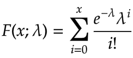
For a Poisson distribution:
- Mean (expected value): E(X) = λ
- Variance: Var(X) = λ
Examples:
- Number of phone calls received by a call center per hour.
- Number of emails received per day.
- Number of customers entering a store per hour.
- Number of defects in a manufactured product per unit.
- Number of cars passing a certain point on a highway per minute.
It has a relationship with Binomial Distribution. The Poisson distribution can be used as an approximation to the binomial distribution when:
- n (the number of trials in the binomial distribution) is large.
- p (the probability of success in each trial) is small.
In such cases, λ can be approximated as λ = n * p.
# Import Necessary Libraries
from scipy.stats import poisson
import numpy as np
numargs = poisson.numargs
a, b = 0.2, 0.8
randomVariable = poisson (a, b)
print ("Random Variable : \n", randomVariable)
quantile = np.arange (0.01, 1, 0.1)
# Random Variates
R = poisson.rvs(a, b, size = 10)
print ("Random Variates : \n", R)
# PDF
x = np.linspace(poisson.ppf(0.01, a, b),
 poisson.ppf(0.99, a, b), 10)
R = poisson.ppf(x, 1, 3)
print ("\nProbability Distribution : \n", R)
Here is the output:
Random Variates : [0 0 0 0 1 0 0 0 0 0] Probability Distribution : [ 5. nan nan nan nan nan nan nan nan nan]
Now let's try to display it graphically
# Import Necessary Libraries
import numpy as np
import matplotlib.pyplot as plt
distribution = np.linspace(0, np.minimum(randomVariable.dist.b, 2))
print("Distribution : \n", distribution)
plot = plt.plot(distribution, randomVariable.ppf(distribution)) 
Here is the Github link for the code - PoissonDistribution.ipynb
Finally, The Bernoulli Distribution
The Bernoulli distribution is the probability distribution of a random variable that can take only two possible outcomes, typically labeled as "success" and "failure".
The Probability Mass Function (PMF) of a Bernoulli distribution is defined as:
- P(X = 1) = p (Probability of success)
- P(X = 0) = q = 1 - p (Probability of failure)
Where X is the random variable representing the outcome of the Bernoulli trial.
- Mean (expected value): E(X) = p
- Variance: Var(X) = p * (1 - p) = p * q
Examples:
- Coin Flip: Flipping a coin once.
Getting heads can be considered a "success" (X = 1), and getting tails can be considered a "failure" (X = 0). If it's a fair coin, p = 0.5. - Medical Test: A patient taking a medical test that has only two outcomes: positive (disease present, X = 1) or negative (disease absent, X = 0).
p would represent the probability of testing positive. - Product Inspection: Inspecting a single product to determine if it's defective (X = 1) or not defective (X = 0).
p represents the probability of a product being defective.
The Bernoulli distribution is a special case of the binomial distribution where the number of trials n is equal to 1.
import numpy as np
import matplotlib.pyplot as plt
import seaborn as sns
def plot_bernoulli(p):
 """
 Plots the probability mass function (PMF) of a Bernoulli distribution.
 Args:
 p: The probability of success (0 <= p <= 1).
 """
 if not (0 <= p <= 1):
 raise ValueError("Probability p must be between 0 and 1.")
 # Possible outcomes (0 for failure, 1 for success)
 outcomes = [0, 1]
 probabilities = [1 - p, p]
 # Create the plot
 plt.figure(figsize=(8, 6))  # Adjust figure size for better visualization
 sns.barplot(x=outcomes, y=probabilities, palette=['skyblue', 'salmon'])
 plt.xticks(outcomes, ['Failure (0)', 'Success (1)']) #More descriptive x-ticks
 plt.xlabel("Outcome")
 plt.ylabel("Probability")
 plt.title(f"Bernoulli Distribution (p = {p})")
 plt.ylim(0, 1) #Set y-axis limits for better visualization
 for i, prob in enumerate(probabilities):
 plt.text(i, prob + 0.01, f"{prob:.2f}", ha='center') #Add probability values above bars
 plt.show()
# Example usage:
p_values = [0.2, 0.5, 0.8] #Different probabilities of success
for p in p_values:
 plot_bernoulli(p)


Here is the Github link for the code - BernoulliDistribution.ipynb
Conclusion
In this blog post, I have explained 4 important Probability distributions with examples. In addition, I have shared the Python code to graphically display them as well.
Disclaimer
This article is not endorsed by Salesforce, Google, or any other company in any way. I shared my knowledge on this topic in this blog post. Please always refer to Official Documentation for the latest information.


0 Comments