A New Year Promise From “technical potpourri”

A New Year Promise From “technical potpourri”

Sudipta Deb

Sudipta Deb

Founder of Technical Potpourri, Co-Founder of Shrey Tech, Enterprise Cloud Architect

Happy New Year, everyone! As the confetti settles and we embark on a fresh new year, I'm thrilled to officially announce the growth of something I've been passionately working on: Technical Potpourri, a space dedicated to exploring the fascinating world of technology in all its diverse and exciting forms.

Think of it as a digital melting pot where we'll delve into a wide range of technical topics, from the fundamentals of programming and data science to the latest advancements in AI, Salesforce, Google Cloud, and beyond. Whether you're a seasoned techie, a curious beginner, or simply someone who wants to stay informed about the ever-evolving tech landscape, I hope you'll find something of interest here.

The form you have selected does not exist.

Why "Technical Potpourri"?

The name reflects the diverse nature of the content. A potpourri is a mixture of various things, and that's exactly what you'll find here: a blend of different technical topics, perspectives, and learning styles.

What To Expect From Technical Potpourri

This isn't your typical dry, technical manual. I aim to make complex concepts accessible and engaging for everyone. Here’s what you can look forward to:

  • Blog Posts: In-depth articles exploring various technical subjects, breaking down complex ideas into digestible pieces. I'll cover everything from coding tutorials and explanations of key algorithms to discussions of emerging technologies and their impact on our lives.
  • YouTube Videos: Complementary video content in the youtube channel that brings the blog posts to life. Expect tutorials, demonstrations, and visual explanations that make learning even more interactive and fun. Think coding walkthroughs, software demos, and explainer videos on complex topics.
  • A Focus on Clarity and Understanding: My goal is to demystify technology, not to intimidate anyone with jargon. I'll strive to explain concepts clearly and concisely, using real-world examples and analogies.
  • A Welcoming Community: I envision Technical Potpourri as a place for learning, discussion, and collaboration. I encourage you to leave comments, ask questions, and share your own experiences.

Growth of "technical potpourri" Blog

I initiated this blog in 2014 as a platform to disseminate my knowledge to a broader audience globally. Over the past decade, there have been fluctuations, although the concept of "technical potpourri" has consistently remained a guiding vision for me. I am pleased to announce that I have published 361 articles on various technical subjects as of today. The subscriber count reached approximately 6,000 during the past decade. I sincerely appreciate your support, suggestions, and efforts to identify avenues for improvement. I trust you will persist, as it has significant importance to me.

Growth of "technical potpourri" YouTube Channel

The YouTube channel "Technical Potpourri" was established subsequently, around November 2020. Over the past four years, I have released 159 videos on various subjects, resulting in about 2.6K subscribers for my family. On December 13th, the channel achieved 275,000 unique views. I am exceedingly proud of the global acceptance I have gotten.

What's Coming Soon:

In the coming weeks and months, you can expect blog posts and videos on topics such as:

  • Tutorials, New Features, and Best Practices around Salesforce
  • Tutorials on Python Programming.
  • Fundamentals of Data Science and Machine Learning.
  • Tutorials, New Features, and Best Practices around Google Cloud
  • Exploring the world of Generative AI.
  • And much more!

Join the Journey!

I'm incredibly excited to embark on this journey with you. I believe that technology has the power to transform our world, and I hope that Technical Potpourri can play a small part in helping people understand and harness that power.

I encourage you to subscribe to the YouTube channel and bookmark the blog to stay updated on the latest content.

Thank you for joining me, and here's to a fantastic and technically enriching new year!

Disclaimer

This article is not endorsed by Salesforce, Google, or any other company in any way. I shared my knowledge on this topic in this blog post. Please always refer to Official Documentation for the latest information.

Comments

4 Important Probability Distributions – Normal, Binomial, Poisson, Bernoulli

4 Important Probability Distributions – Normal, Binomial, Poisson, Bernoulli

Sudipta Deb

Sudipta Deb

Founder of Technical Potpourri, Co-Founder of Shrey Tech, Enterprise Cloud Architect

A probability distribution specifies the likelihood of all possible outcomes of a random variable. The distribution may be classified as either continuous or discrete based on the values assumed by a random variable. Various forms of probability distributions exist. In this post, I will examine Normal, Binomial, Poisson and Bernoulli distribution and demonstrate how to utilize Python to plot it.

Regardless of your domain, Statistics and Probability will be there. Economics, finance, trading, social sciences, natural sciences, and data science are essential. A substantial portion of data science involves comprehending the behaviors and characteristics of variables, which necessitates knowledge of their corresponding distributions. The probability distribution is a method to depict the potential values a variable may assume along with their corresponding probabilities.

In this blog post, I will show you how to use the Python programming language to plot these 4 distributions.

The form you have selected does not exist.

Let's Understand Probability Distribution 

A probability distribution is a function in probability theory and statistics that quantifies the likelihood of various outcomes in an experiment. It delineates occurrences based on their probability relative to all potential outcomes.

Let's say, the probability distribution of a fair coin toss. Heads takes a value of X = 0.5 and tails gets X = 0.5 too.

Understand Density Function

Another important thing to understand is the density function. The density functions are mathematical functions that describe the probability distribution of a random variable X. We have two density functions - Probability Mass Function (PMF) and Probability Density Function (PDF).

Probability Mass Function (PMF)

Describes the probability distribution of a discrete random variable. Discrete variables are those that can only take on a finite number of values or a countably infinite number of values (e.g., 0, 1, 2, 3...). Examples:

  • The number of heads in 3 coin flips (can be 0, 1, 2, or 3).
  • The number of cars passing a point on a road in an hour.

Probability Density Function (PDF)

Describes the probability distribution of a continuous random variable. Continuous variables can take on any value within a given range (e.g., any real number between 0 and 1). Examples:

  • The temperature of city.
  • A person's weight.
  • The time it takes to fix a bug.

Let's Start With Normal Distribution

The Normal Distribution is a probability distribution that is symmetric around its mean value. It is a continuous distribution with two parameters: mean (μ) and standard deviation (σ). The bell-shaped curve of the Normal Distribution shows that most of the data falls near the mean, while the tail shows that there is still a chance for data to fall from the mean.

I have written a dedicated blog post covering Normal Distribution. So instead of duplicating the content, I am linking the blog post where you can get all the details you need about Normal Distribution. 

Blog Post - Normal Distribution Using Python and SciPy

GitHub Code - NormalDistribution.ipynb

Now It's Time For Binomial Distribution

The binomial distribution is a discrete probability distribution that describes the probability of obtaining a certain number of successes in a sequence of independent experiments, each having only two possible outcomes: success or failure.

The binomial distribution is based on a series of independent trials called Bernoulli trials. Each Bernoulli trial has only two possible outcomes, conventionally labeled "success" and "failure." The probability of success is denoted by p, and the probability of failure is denoted by q = 1 - p. The probability p remains constant for each trial.

A binomial experiment consists of a fixed number (n) of independent Bernoulli trials. The binomial random variable X represents the number of successes in n Bernoulli trials.

The probability of getting exactly k successes in n trials is given by the binomial PMF:

Binomial distribution function

Where:

  • P(x): Binomial Probability
  • nCx is the binomial coefficient, also written as "n choose x," which represents the number of ways to choose x successes from n trials.
  • x: Number of times for a specific outcome within n trials
  • p: Probability of success on a single trial
  • q: Probability of failure on a single trial
  • n: Number of trials

Binomial Distribution has the below values:

  • Mean: μ = n * p
  • Standard Deviation: n * p * q = n * p * (1 - p)

Example:

  • Coin Flips: Flipping a fair coin 10 times and counting the number of heads. Here, n = 10, and p = 0.5 (assuming a fair coin).
  • Quality Control: Inspecting a batch of 100 products and counting the number of defective items. Here, n = 100, and p would be the probability of a single product being defective.
  • Medical Testing: Testing 50 patients for a disease and counting the number of positive results. Here, n = 50, and p would be the prevalence of the disease in the population.

 Here comes the code

# Import Necessary Libraries
from scipy.stats import binom 
# Setting up all the parameters
n = 6
p = 0.6
# defining the list of possible values
possible_values = list(range(n + 1)) 
# Get the mean and variance
mean, var = binom.stats(n, p) 
# Get All PMF Values
all_pmf_values = [binom.pmf(outcome, n, p) for outcome in possible_values ] 
# Printing the Outcome and Probability
print("Outcome\tP(X)") 
for i in range(n + 1): 
 print(str(possible_values[i]) + "\t" + str(all_pmf_values[i])) 
# Printing Mean and Variance
print("Mean = "+str(mean)) 
print("Variance = "+str(var))

Now plotting it as vertical bar 

# Import Necessary Libraries
from scipy.stats import binom 
import matplotlib.pyplot as plt 
# Setting up all the parameters 
n = 6
p = 0.6
# defining the list of possible values
possible_values = list(range(n + 1)) 
# Get All PMF Values
all_pmf_values = [binom.pmf(r, n, p) for r in possible_values ] 
# plotting the graph 
plt.bar(possible_values, all_pmf_values) 
plt.show()

Here is the graph

When probability of success and failure are same (equally likely), the binomial distribution becomes a normal distribution. So changing the
value of p to 0.5, the graph will become a normal distribution

Here is the Github link for the code - BinomialDistribution.ipynb

Time For Poisson Distribution

The Poisson distribution is a discrete probability distribution that describes the probability of a given number of events occurring in a fixed interval of time or space if these events occur with a known average rate and independently of the time since the last event. The Poisson distribution is applicable when the following conditions are met:

  • Events are independent: The occurrence of one event does not affect the probability of another event occurring.
  • Events occur at a constant average rate: The average number of events per unit of time or space is constant. This average rate is denoted by λ (lambda).
  • Events occur randomly: Events occur randomly and uniformly within the interval.
  • The probability of two or more events occurring in a very short interval is negligible.

The Probability Mass Function for Poisson distribution is given by

Poisson Distribution | Probability Distributions

Here, lambda is the shape parameter that describes the average number of events in that interval.

lambda is also the mean and variance of the distribution.

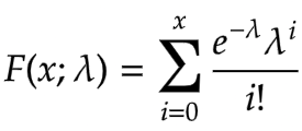
The cumulative distribution function is given as

cumulative distribution function | Probability Distributions

For a Poisson distribution:

  • Mean (expected value): E(X) = λ
  • Variance: Var(X) = λ

Examples:

  • Number of phone calls received by a call center per hour.
  • Number of emails received per day.
  • Number of customers entering a store per hour.
  • Number of defects in a manufactured product per unit.
  • Number of cars passing a certain point on a highway per minute.

It has a relationship with Binomial Distribution. The Poisson distribution can be used as an approximation to the binomial distribution when:

  • n (the number of trials in the binomial distribution) is large.
  • p (the probability of success in each trial) is small.

In such cases, λ can be approximated as λ = n * p.

# Import Necessary Libraries
from scipy.stats import poisson 
import numpy as np 
numargs = poisson.numargs 
a, b = 0.2, 0.8
randomVariable = poisson (a, b) 
print ("Random Variable : \n", randomVariable) 
quantile = np.arange (0.01, 1, 0.1) 
# Random Variates 
R = poisson.rvs(a, b, size = 10) 
print ("Random Variates : \n", R) 
# PDF 
x = np.linspace(poisson.ppf(0.01, a, b), 
 poisson.ppf(0.99, a, b), 10) 
R = poisson.ppf(x, 1, 3) 
print ("\nProbability Distribution : \n", R) 

Here is the output:

Random Variates : [0 0 0 0 1 0 0 0 0 0] Probability Distribution : [ 5. nan nan nan nan nan nan nan nan nan]

Now let's try to display it graphically

# Import Necessary Libraries
import numpy as np 
import matplotlib.pyplot as plt 
distribution = np.linspace(0, np.minimum(randomVariable.dist.b, 2)) 
print("Distribution : \n", distribution) 
plot = plt.plot(distribution, randomVariable.ppf(distribution)) 

Here is the Github link for the code - PoissonDistribution.ipynb

Finally, The Bernoulli Distribution

The Bernoulli distribution is the probability distribution of a random variable that can take only two possible outcomes, typically labeled as "success" and "failure". It's the simplest discrete probability distribution and serves as the foundation for other distributions like the binomial distribution. The Bernoulli distribution models a single trial or experiment with only two possible outcomes. This trial is called a Bernoulli trial. Success: Usually represented by the value 1. The probability of success is denoted by p. Failure:Usually represented by the value 0.The probability of failure is denoted by q, where q = 1 - p.

The Probability Mass Function (PMF) of a Bernoulli distribution is defined as:

  • P(X = 1) = p (Probability of success)
  • P(X = 0) = q = 1 - p (Probability of failure)

Where X is the random variable representing the outcome of the Bernoulli trial.

  • Mean (expected value): E(X) = p
  • Variance: Var(X) = p * (1 - p) = p * q

Examples:

  • Coin Flip: Flipping a coin once. Getting heads can be considered a "success" (X = 1), and getting tails can be considered a "failure" (X = 0). If it's a fair coin, p = 0.5.
  • Medical Test: A patient taking a medical test that has only two outcomes: positive (disease present, X = 1) or negative (disease absent, X = 0). p would represent the probability of testing positive.
  • Product Inspection: Inspecting a single product to determine if it's defective (X = 1) or not defective (X = 0). p represents the probability of a product being defective.

The Bernoulli distribution is a special case of the binomial distribution where the number of trials n is equal to 1. In other words, a binomial distribution describes the number of successes in multiple independent Bernoulli trials.

import numpy as np
import matplotlib.pyplot as plt
import seaborn as sns
def plot_bernoulli(p):
 """
 Plots the probability mass function (PMF) of a Bernoulli distribution.
 Args:
 p: The probability of success (0 <= p <= 1).
 """
 if not (0 <= p <= 1):
 raise ValueError("Probability p must be between 0 and 1.")
 # Possible outcomes (0 for failure, 1 for success)
 outcomes = [0, 1]
 probabilities = [1 - p, p]
 # Create the plot
 plt.figure(figsize=(8, 6))  # Adjust figure size for better visualization
 sns.barplot(x=outcomes, y=probabilities, palette=['skyblue', 'salmon']) 
 plt.xticks(outcomes, ['Failure (0)', 'Success (1)']) #More descriptive x-ticks
 plt.xlabel("Outcome")
 plt.ylabel("Probability")
 plt.title(f"Bernoulli Distribution (p = {p})")
 plt.ylim(0, 1) #Set y-axis limits for better visualization 
 for i, prob in enumerate(probabilities):
 plt.text(i, prob + 0.01, f"{prob:.2f}", ha='center') #Add probability values above bars
 plt.show()
# Example usage:
p_values = [0.2, 0.5, 0.8] #Different probabilities of success
for p in p_values:
 plot_bernoulli(p)

Here is the Github link for the code - BernoulliDistribution.ipynb

Conclusion

In this blog post, I have explained 4 important Probability distributions with examples. In addition, I have shared the Python code to graphically display them as well.

Disclaimer

This article is not endorsed by Salesforce, Google, or any other company in any way. I shared my knowledge on this topic in this blog post. Please always refer to Official Documentation for the latest information.

Comments

Calculate Z-Score in Python

Calculate Z-Score in Python

Sudipta Deb

Sudipta Deb

Founder of Technical Potpourri, Co-Founder of Shrey Tech, Enterprise Cloud Architect

A Z-score, or standard score, indicates the distance of a data point from the mean. More formally, it quantifies the number of standard deviations a raw score deviates from the population mean.

A Z-score can be positioned on a normal distribution curve. To calculate a Z-score, it is essential to know the mean μ and the population standard deviation σ. These scores range from -3 standard deviations (which would fall to the far left of the normal distribution curve) up to +3 standard deviations (which would fall to the far right of the normal distribution curve).

Z-scores are a way to compare results to a “normal” population. Results from tests or surveys have thousands of possible results and units; those results can often seem meaningless. For example, knowing that someone’s earning is 100 K dollar might be good information, but if you want to compare it to the “average” person’s earning, looking at a vast table of data can be overwhelming. The scores can tell you where that person’s earning is compared to the average population’s mean earning.

The form you have selected does not exist.

Sample Code

I normally put all my codes in my personal Github repository, so that I can easily share with others. Here is the Github Code Repo where you can find the code samples used in this blog post.

Z-Score.ipynb

Let's Understand The Problem Statement

Suppose we know that the GRE scores are normally distributed with mean 157 and standard deviation 17 and IELTS scores are normally distributed with mean 6.8 and standard devialtion 1.2.

A university provides admission to their courses only on the basis of GRE and IELTS scores. The college admission committee decided to give the top performer scholarship to the student who has performed the best among all applicants. The highest score received from applicants who appeared for GRE is 182 and the highest score received from applicants who appeared for IELTS is 9.

What should be the strategy for the college to find the best candidate!

Let's First Visualize The Data

# Plot the two distribution for GRE and IELTS
from scipy.stats import norm
import matplotlib.pyplot as plt
import numpy as np
fig, (ax1, ax2) = plt.subplots(1,2,figsize=(15,5))
x=np.linspace(20,300,500)
ax1.plot(x,norm.pdf(x,157,17),color="b")
ax1.set_title("GRE")
ax1.set_xlabel("GRE Score")
ax1.set_ylabel("Probability")
ax1.axvline(182,linestyle="--",color="green")
x1=np.linspace(2,10,500)
ax2.plot(x1,norm.pdf(x1,6.8,1.2),color="r")
ax2.set_title("IELTS")
ax2.set_xlabel("IELTS Score")
ax2.set_ylabel("Probability")
ax2.axvline(9,linestyle="--",color="green")
plt.show()

Now The Question Is - How Far From The Mean The Two High Scores Are? i.e. Z-Score

We can find out the Z-Scores in the below way. Remember the formula to find out the Z-Score is - z = (x – μ) / σ

  • μ - Mean Value
  • σ - Standard Deviation
# Find the Z-Score of the hihgest score in GRE and IELTS among all applicants
top_gre = (182 - 157) / 17
print("The Z-Score of the highest score in GRE among all applicants: ",top_gre);
top_ielts = (9 - 6.8) / 1.2
print("The Z-Score of the highest score in IELTS among all applicants: ",top_ielts);

Here is the result -

The Z-Score of the highest score in GRE among all applicants: 1.4705882352941178
The Z-Score of the highest score in IELTS among all applicants: 1.8333333333333335

Now comparing the Z-Scores, it is very much clear that student scored highest in IELTS is definitely higher that the student scored highest in GRE. But let's visualize this in a graph.

Visualize The Z-Score

fig, ax = plt.subplots()
x = np.linspace(-2,2,50)
ax.plot(x,norm.pdf(x,0,1),color="b")
ax.set_title("Standard Normal Distribution")
ax.set_xlabel("Z-Score")
ax.set_ylabel("Probability")
ax.axvline(top_gre,linestyle="--",color="green")
ax.axvline(top_ielts,linestyle="--",color="red")
plt.show()

From the graph also it is very clear that student who scored highest in IELTS is definitly the student who should receive the scholarship from the University.

Interpretation Of Z-Score

  • Z-Score = 0: A Z-score of 0 indicates that the data point is exactly at the mean of the distribution.
  • Positive Z-Score: A positive Z-score indicates that the data point is above the mean. For example, a Z-score of 2.5 means the data point is 2.5 standard deviations above the mean.
  • Negative Z-Score: A negative Z-score indicates that the data point is below the mean. For example, a Z-score of -3.7 means the data point is 3.7 standard deviations below the mean.
  • Magnitude of Z-Score: The magnitude of the Z-score shows how far away the data point is from the mean. A larger absolute value of the Z-score indicates that the data point is farther from the mean, while a smaller absolute value indicates it is closer.

What Is 68-95-99.7 Rule In Relation To Z-Scores?

The 68-95-99.7 Rule, also known as the Empirical Rule, states that:

  • About 68% of data falls within 1 standard deviation from the mean.
  • About 95% falls within 2 standard deviations.
  • About 99.7% falls within 3 standard deviations.

Conclusion

Z-score is an essential statistical tool that provides a standardized measure of how a data point deviates from the mean of a distribution. Its is employed in different industries, including finance, education, health, and engineering, making it a versatile tool for data analysis. By translating raw data into a standardized scale, Z-scores assist the comparison of diverse datasets and the identification of outliers. This uniformity is vital for statistical testing, quality control, and risk management. Understanding how to compute and understand Z-scores enables for more effective data analysis and decision-making.

Disclaimer

This article is not endorsed by Salesforce, Google, or any other company in any way. I shared my knowledge on this topic in this blog post. Please always refer to Official Documentation for the latest information.

Comments

Detect Outliers Using Z-Score In Python

Detect Outliers Using Z-Score In Python

Sudipta Deb

Sudipta Deb

Founder of Technical Potpourri, Co-Founder of Shrey Tech, Enterprise Cloud Architect

A Z-score, or standard score, indicates the distance of a data point from the mean. More formally, it quantifies the number of standard deviations a raw score deviates from the population mean.

A Z-score can be positioned on a normal distribution curve. To calculate a Z-score, it is essential to know the mean μ and the population standard deviation σ. These scores range from -3 standard deviations (which would fall to the far left of the normal distribution curve) up to +3 standard deviations (which would fall to the far right of the normal distribution curve).

Z-scores are a way to compare results to a “normal” population. Results from tests or surveys have thousands of possible results and units; those results can often seem meaningless. For example, knowing that someone’s earning is 100 K dollar might be good information, but if you want to compare it to the “average” person’s earning, looking at a vast table of data can be overwhelming. The scores can tell you where that person’s earning is compared to the average population’s mean earning.

I have published a dedicated post covering the topic Z-Score. If you want to know in details about Z-Score, I would highly recommend going through that post first. Link is given below.

Calculate Z-Score in Python

The form you have selected does not exist.

Sample Code

I normally put all my codes in my personal Github repository, so that I can easily share with others. Here is the Github Code Repo where you can find the code samples used in this blog post.

OutliersUsingZ-Score.ipynb

Z-Score And Outliers

In a Normal Distribution, it is estimated that 68% of the data points lie between +/- 1 standard deviation, 95% of the data points lie between +/- 2 standard deviation, 99.7% of the data points lie between +/-3 standard deviation.

Now if the Z-Score of a data point is more than 3, it indicates that the data point is quite different from rest of the data points. Such a data points are called Outliers.

Calculate Outliers Using Z-Score 

import numpy as np
data = [1,1,2,2,1188,2,3,4,1,2,2]
print(data)
mean = np.mean(data)
standard_deviation = np.std(data)
print('Mean: ',mean)
print("Standard Deviation: ", standard_deviation)

Output:

[1, 1, 2, 2, 1188, 2, 3, 4, 1, 2, 2]
Mean: 109.81818181818181
Standard Deviation: 340.95209425740796

# Find the Outliers
threshold = 3
outliers = []
for index in data:
 z_score = (index - mean) / standard_deviation
 if(z_score >= threshold):
 outliers.append(index)
print(outliers)

Output:

[1188]

So, we can easilly see that number 1188 is the outlier in the dataset.

Disclaimer

This article is not endorsed by Salesforce, Google, or any other company in any way. I shared my knowledge on this topic in this blog post. Please always refer to Official Documentation for the latest information.

Comments

Normal Distribution Using Python and SciPy

Normal Distribution Using Python and SciPy

Sudipta Deb

Sudipta Deb

Founder of Technical Potpourri, Co-Founder of Shrey Tech, Enterprise Cloud Architect

Scipy Stats Norm is a component of Scipy Stats utilized for manipulating the normal distribution. The normal distribution is a significant statistical distribution extensively utilized across diverse domains, including finance, physics, and engineering.

Scipy Statistics Norm offers several methods for analyzing the normal distribution, encompassing probability density functions, cumulative distribution functions, and random number generation. These tools facilitate developers' engagement with the standard distribution in Python.

This blog post will elucidate the fundamentals of Scipy Stats Norm and its effective application. I will begin by examining the probability density function and its application in calculating probabilities. Subsequently, I will examine the cumulative distribution function and its application in calculating percentiles. Ultimately, I will examine random number generation and its use in producing random numbers from a normal distribution.

The form you have selected does not exist.

Sample Code

I normally put all my codes in my personal Github repository, so that I can easily share with others. Here is the Github Code Repo where you can find the code samples used in this blog post.

NormalDistribution.ipynb

What Is Normal Distribution?

The Normal Distribution is a probability distribution that is symmetric around its mean value. It is a continuous distribution with two parameters: mean (μ) and standard deviation (σ). The bell-shaped curve of the Normal Distribution shows that most of the data falls near the mean, while the tail shows that there is still a chance for data to fall from the mean.

Normal Distribution Using SciPy

Scipy Stats Norm is a submodule of Scipy library that provides methods for working with Normal Distribution. We can use it to create a Normal Distribution with given mean and standard deviation values. We can use the returned object (normal_distribution) to perform various operations related to normal distribution.

# Creating Normal Distribution
# Load SciPy's Statistical Model
from scipy import stats
# Create Mean and Standard Deviation
mean = 35
standard_deviation = 7.2
# Create Normal Distribution
# loc - Mean Value 
# scale - Standard Deviation Value
normal_distribution = stats.norm(
 loc = mean,
 scale = standard_deviation
)

Probability Of A Given Value Using pdf()

We can find out the answer to this question - What is the probability that the value is 40? The method pdf() from the norm class can help us to answer this question. It returns the probabilities for specific values from a normal distribution.

PDF = Probability Distribution Function

# Use PDF to understand what is the probability that the value is 40 in this normal distribution
pdf = normal_distribution.pdf(40)
print(pdf)

The result is: 8.27133. So that means there is a  8.27133% chance that a randomly selected number has value 40.

Density Curve Using pdf()

A density curve is a graphical plot showing probabilities associated with different values of a variable. We can use pdf() to plot the density curve for the values.

First, we will pick evenly spaced 1000 numbers between 10 and 990.

# Pick some equally spaced 1000 bnumbers between 10 and 990
# Load numpy
import numpy as np
min_value = 10
max_value = 990
equally_spaced_values = np.linspace(min_value, max_value, 1000)
# Let's print the size, first 10 and last 10 values
print("Size: ", equally_spaced_values.size)
print("First 10 Values: ", equally_spaced_values[:10].round(2))
print("Last 10 Values: ", equally_spaced_values[-10:].round(2))

Here comes the output:

Size: 1000

First 10 Values: [10. 10.98 11.96 12.94 13.92 14.9 15.89 16.87 17.85 18.83]

Last 10 Values: [981.17 982.15 983.13 984.11 985.1 986.08 987.06 988.04 989.02 990. ]

Now, we can get the probabilities of all these values using pdf() function.

# Probability of all values
all_probabilities = normal_distribution.pdf(x=equally_spaced_values)
print(all_probabilities)

Finally, we can plot the value along X-Axis and the corresponding probabilities along Y-Axis. This will give us the density curve.

# Density Curve
# Set grapph size
from matplotlib import pyplot as plt  plt.figure(figsize=(20, 12))
plt.plot(equally_spaced_values, all_probabilities)
plt.fill_between(equally_spaced_values, all_probabilities, color="r")
axes=plt.gca()
axes.set_xlim([min_value, max_value])
plt.xlabel("Values")
plt.ylabel("Probabilities")
plt.title("Density Curve")
plt.show()

Find Percent Values Below a Value

Now the question is - What is the percentage that selected number has value less than 450?

To answer this question, we need to add the probabilities of all values less than 450. The norm method cdf() will be able to do that. This method calculated the proportion of a normally distributed population that is less than or equal to a given value.

CDF = Cumulative Distribution Function.

# How many numbers has value less than 450?
less_than_450 = normal_distribution.cdf(450)
print(less_than_450)

Output is: 0.21652. This means 0.21652% of records have values less than 450.

Visualize It

We can definitely visualize it by the below way

# Set graph size
plt.figure(figsize=(20, 12))
# plot density function
plt.plot(equally_spaced_values, all_probabilities)
plt.axvline(x=450, color="red")
#Shade the region where the value is less than equal to 450
x1 = np.linspace(equally_spaced_values.min(), 450, 100)
plt.fill_between(x1, norm.pdf(x1, mean, standard_deviation), color="r")
# Remove the dead space
axes = plt.gca()
axes.set_xlim([min_value, max_value])
ymin, ymax = axes.get_ylim()
axes.set_ylim([0, ymax])
plt.title("Value is less than equal 40")
plt.xlabel("Values")
plt.ylabel("Probabilities")
plt.show()

Find Percent Values Above a Value

If the question is - What is the probability that a randomly selected number has a value greater than 450?

To calculate this, we need to subtract the probability that a randomly selected number is less than or equal to 450 from 1. Why 1? The reason is the sum of all probabilities is always 1.

# How many numbers has value less than 450?
less_than_450 = normal_distribution.cdf(450)
print(less_than_450)

Since the output is 0.78345, that means there is a 0.78345% chance that the selected number has a value greater than 450.

Let's Visualize It

# Set graph size
plt.figure(figsize=(20, 12))
# plot density function
plt.plot(equally_spaced_values, all_probabilities)
plt.axvline(x=450, color="red")
#Shade the region where the value is less than equal to 450
x1 = np.linspace(450, equally_spaced_values.max(), 100)
plt.fill_between(x1, norm.pdf(x1, mean, standard_deviation), color="r")
# Remove the dead space
axes = plt.gca()
axes.set_xlim([min_value, max_value])
ymin, ymax = axes.get_ylim()
axes.set_ylim([0, ymax])
plt.title("Value is less than equal 40")
plt.xlabel("Values")
plt.ylabel("Probabilities")
plt.show()

Calculate Percentile Using ppf()

Let's say this time you want to find the min value so that 90% of all values are greater than that value. In general, this is called percentile. The Nth percentile is the value that is greater than the N percent of all data points.

We can use the ppf() function to find that value.

PPF = Percent Point Function.

# Find the min value so that 90% of all values are greater than that value
percentile_90th = normal_distribution.ppf(0.9)
print(percentile_90th)

Output is: 708.1939. It means 708.1939 is the min value to make sure 90% of all values are greater than this.

Visualize It

# Let's Visualize It
plt.plot(equally_spaced_values, all_probabilities)
plt.axvline(x=percentile_90th, color="red")
plt.xlabel("Values")
plt.ylabel("Probabilities")
plt.show()

Conclusion

I hope this blog post helped you gain practical skills using Python and SciPy. Let’s do a quick recap of what you’ve learned:

  • Create normal distributions using the norm class from the SciPy stats module.
  • Generate random samples using the norm method rvs().
  • Calculate probabilities using pdf() and cdf().
  • Find percentiles using ppf().
  • Plot histogram and density curve for normal distributions using Matplotlib and Seaborn.

Disclaimer

This article is not endorsed by Salesforce, Google, or any other company in any way. I shared my knowledge on this topic in this blog post. Please always refer to Official Documentation for the latest information.

Comments